Short Introduction to BAMP

Volker Schmid

2026-08-08

Introduction

Age-period-cohort (APC) models decompose incidence or mortality rates into three smooth components: an age effect (how risk varies across age groups), a period effect (how risk varies over calendar time) and a cohort effect (how risk varies across birth cohorts). BAMP fits such models in a Bayesian framework via MCMC and provides tools to check convergence, inspect the fitted effects, and predict future cases.

Data example

BAMP includes a data example: cases and population, matrices of observed case counts and population at risk, cross-classified by calendar year (rows) and age group (columns).

data(apc)
plot(cases[,1],type="l",ylim=range(cases), ylab="cases", xlab="year", main="cases per age group")
for (i in 2:8)lines(cases[,i], col=i)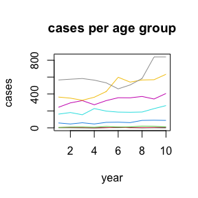

For simulating your own APC data, see vignette(“simulation”, package=“bamp”).

APC model with random-walk first-order priors

We fit a model with a first-order random walk ("rw1") prior on each of the age, period and cohort effects – a common default that assumes each effect changes smoothly, without a systematic trend, between neighbouring levels. periods_per_agegroup tells bamp() how many calendar years each age group spans, which is needed to map age and period onto the cohort dimension.

model1 <- bamp(cases, population, age="rw1", period="rw1", cohort="rw1",
              periods_per_agegroup = 5)

bamp() automatically checks MCMC convergence using the Gelman-Rubin diagnostic and warns if the chains have not converged. We can also run this check manually:

checkConvergence(model1)

## [1] TRUE

print() summarises the fitted model: posterior estimates of the smoothing (precision) parameters, and the deviance and DIC, which are useful for comparing models (see vignette(“modeling”, package=“bamp”) for model selection):

print(model1)

## 
##  Model:
## age (rw1)  - period (rw1)  - cohort (rw1) model
## 
##  Effects:            5%           50%          95%         
## intercept                   -10.511      -10.446      -10.387
## 
## Deviance:     230.12
## pD:            36.60
## DIC:          266.72
## 
## 
##  Hyper parameters:                 5%           50%          95%         
## age                              0.436        1.108        2.295
## period                          48.842      128.964      320.787
## cohort                          35.190       61.080      103.190
## 
## 
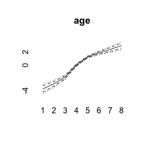
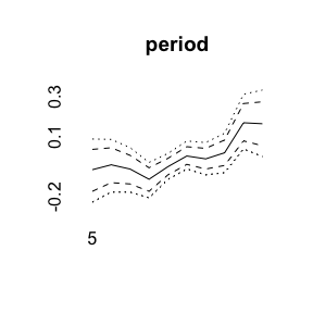
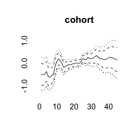
## Markov Chains convergence checked succesfully using Gelman's R (potential scale reduction factor).

The fitted age, period and cohort effects can be plotted with point-wise posterior quantiles:

plot(model1)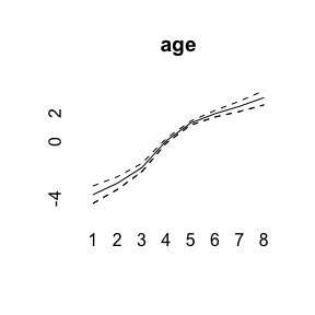

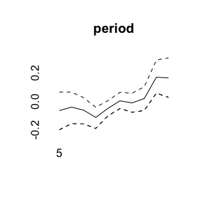
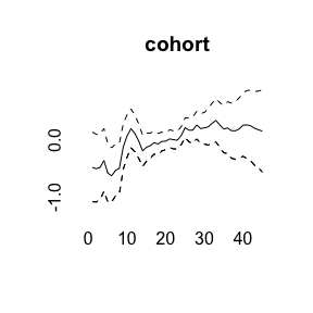
By default the plot shows the median and a 90% interval; other quantiles can be requested explicitly:

plot(model1, quantiles = c(0.025,0.1,0.5,0.9,0.975))

For other prior choices (e.g. second-order random walks, heterogeneity, covariates), see vignette(“modeling”, package=“bamp”).

Prediction

Because the period and cohort effects are modelled as random walks, their most likely continuation is a flat extrapolation with growing uncertainty – which lets us predict cases for upcoming years:

pred <- predict_apc(object=model1, periods=3)

The plot below shows the predicted probability of a case per age group; the dashed vertical line marks the start of the 3-year forecast:

m<-max(pred$pr[2,,])
plot(pred$pr[2,,8],type="l", ylab="probability", xlab="year", ylim=c(0,m))
for (i in 7:1)
  lines(pred$pr[2,,i],col=8-i)
legend(1,m,col=8:1,legend=paste("Age group",1:8),lwd=2,cex=0.6)
lines(c(10.5,10.5),c(0,1),lty=2)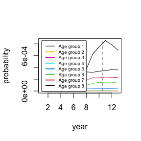

For more details, see vignette(“prediction”, package=“bamp”).