Bayesian Age-Period-Cohort Modeling
Volker Schmid
2026-08-31
Source:vignettes/largevignettes/modeling.Rmd
modeling.RmdThis vignette walks through the range of age-period-cohort (APC)
models that bamp() can fit: different smoothness priors for
the age, period and cohort effects, a model that omits an effect
entirely, and models where the period or cohort effect is scaled by a
known covariate. For a first introduction to bamp(), see
vignette(“bamp”, package=“bamp”); for forecasting, see
vignette(“prediction”, package=“bamp”).
Data example
BAMP includes a data example: cases and
population, matrices of observed case counts and population
at risk, cross-classified by calendar year (rows) and age group
(columns). It also bundles cov_p and cov_c,
example period and cohort covariates used in the last two models
below.
data(apc)
plot(cases[,1],type="l",ylim=range(cases), ylab="cases", xlab="year", main="cases per age group")
for (i in 2:8)lines(cases[,i], col=i)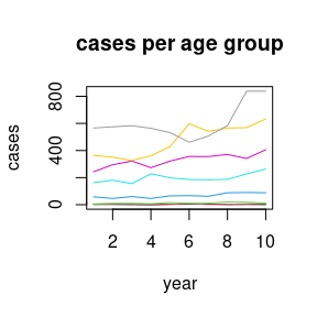
APC model with random-walk first-order priors
A first-order random walk ("rw1") prior assumes each
effect changes smoothly, without a systematic trend, between
neighbouring age groups, periods or cohorts. This is the most common
default.
model1 <- bamp(cases, population, age="rw1", period="rw1", cohort="rw1",
              periods_per_agegroup = 5)
bamp() automatically checks MCMC convergence using the
Gelman-Rubin diagnostic. We can also run this check manually:
checkConvergence(model1)## [1] TRUEprint() summarises the fitted model: posterior estimates
of the smoothing (precision) parameters, and the deviance and DIC, which
are useful for comparing the models fitted in this vignette:
print(model1)##
## Model:
## age (rw1) - period (rw1) - cohort (rw1) model
##
## Effects: 5% 50% 95%
## intercept -10.511 -10.446 -10.387
##
## Deviance: 230.12
## pD: 36.60
## DIC: 266.72
##
##
## Hyper parameters: 5% 50% 95%
## age 0.436 1.108 2.295
## period 48.842 128.964 320.787
## cohort 35.190 61.080 103.190
##
##
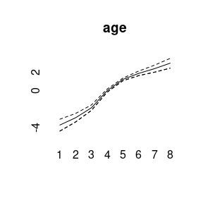
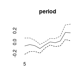
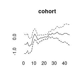
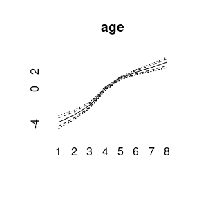
## Markov Chains convergence checked succesfully using Gelman's R (potential scale reduction factor).The fitted age, period and cohort effects can be plotted with point-wise posterior quantiles:
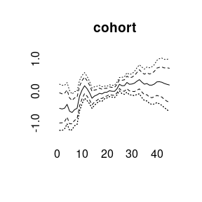
plot(model1)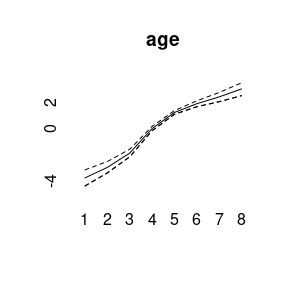
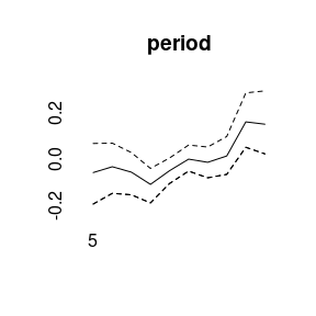
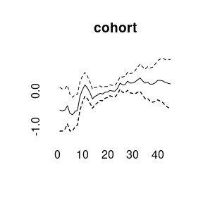
By default the plot shows the median and a 90% interval; other quantiles can be requested explicitly:
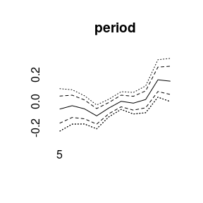
APC model with random-walk second-order priors
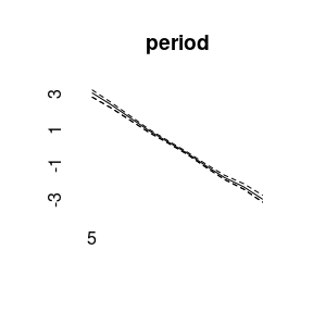
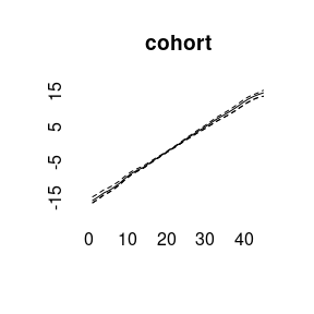
A second-order random walk ("rw2") prior penalises
curvature rather than level, so it produces effects that follow a
smooth, roughly linear trend instead of reverting towards a constant.
RW2 priors are less informative than RW1, so the chains mix more slowly
and need substantially more iterations to converge; here we also set the
smoothing hyperparameters explicitly instead of using the defaults.
model2 <- bamp(cases, population, age="rw2", period="rw2", cohort="rw2",
              periods_per_agegroup = 5,
              mcmc.options=list("number_of_iterations"=200000, "burn_in"=100000, "step"=50, "tuning"=500),
              hyperpar=list("age"=c(1,.5), "period"=c(1,0.05), "cohort"=c(1,0.05)))
checkConvergence(model2)## [1] TRUE
print(model2)##
## Model:
## age (rw2) - period (rw2) - cohort (rw2) model
##
## Effects: 5% 50% 95%
## intercept -10.530 -10.459 -10.394
##
## Deviance: 233.58
## pD: 35.72
## DIC: 269.30
##
##
## Hyper parameters: 5% 50% 95%
## age 1.090 3.024 6.847
## period 16.052 41.275 91.027
## cohort 24.825 46.878 83.398
##
##
## Markov Chains convergence checked succesfully using Gelman's R (potential scale reduction factor).
plot(model2)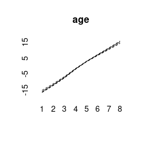
APC model without a period effect
Age, period and cohort are linearly dependent – any one is determined
by the other two – so a model with all three as unrestricted smooth
trends is not identifiable. One common way to sidestep this is to drop
the effect of least interest – here the period effect
(period=" ") – and keep only age and cohort:
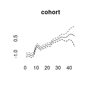
model3<-bamp(cases, population, age="rw1", period=" ", cohort="rw2",
              periods_per_agegroup = 5)
checkConvergence(model3)## [1] TRUE
print(model3)##
## Model:
## age (rw1) cohort (rw2) model
##
## Effects: 5% 50% 95%
## intercept -10.529 -10.456 -10.390
##
## Deviance: 275.82
## pD: 29.69
## DIC: 305.52
##
##
## Hyper parameters: 5% 50% 95%
## age 0.299 0.724 1.497
## cohort 36.892 73.124 139.543
##
##
## Markov Chains convergence checked succesfully using Gelman's R (potential scale reduction factor).
plot(model3)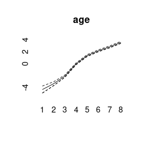
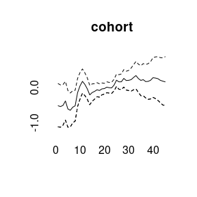
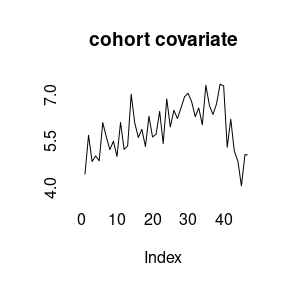
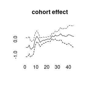
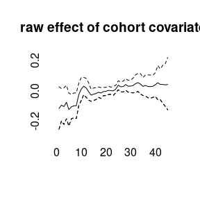
APC model with a cohort covariate
Instead of dropping an effect, a known covariate can scale it:
cohort_covariate multiplies the cohort effect by a given
value at each cohort (here the bundled example covariate
cov_c), which is useful when an external, cohort-specific
risk factor is available.
(model4<-bamp(cases, population, age="rw1", period="rw1", cohort="rw1",
             cohort_covariate = cov_c, periods_per_agegroup = 5))
##
## Model:
## age (rw1) - period (rw1) - cohort (rw1) model
##
## Effects: 5% 50% 95%
## intercept -10.519 -10.451 -10.388
##
## Deviance: 230.43
## pD: 37.39
## DIC: 267.81
##
##
## Hyper parameters: 5% 50% 95%
## age 0.408 1.021 2.101
## period 55.546 142.037 349.491
## cohort 31.623 54.483 92.487
##
##
## Markov Chains convergence checked succesfully using Gelman's R (potential scale reduction factor).
plot(model4)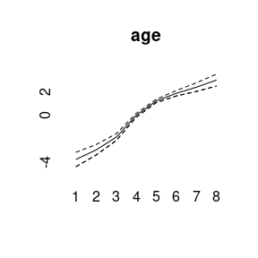
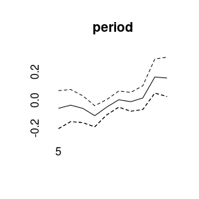
APC model with a period covariate
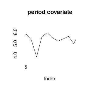
Analogously, period_covariate scales the period effect
by a known, period-specific covariate (here cov_p):
(model5<-bamp(cases, population, age="rw1", period="rw1", cohort="rw1",
             period_covariate = cov_p, periods_per_agegroup = 5))
##
## Model:
## age (rw1) - period (rw1) - cohort (rw1) model
##
## Effects: 5% 50% 95%
## intercept -10.513 -10.447 -10.386
##
## Deviance: 229.64
## pD: 36.71
## DIC: 266.35
##
##
## Hyper parameters: 5% 50% 95%
## age 0.442 1.098 2.226
## period 54.273 147.975 384.812
## cohort 34.560 60.147 98.309
##
##
## Markov Chains convergence checked succesfully using Gelman's R (potential scale reduction factor).
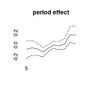
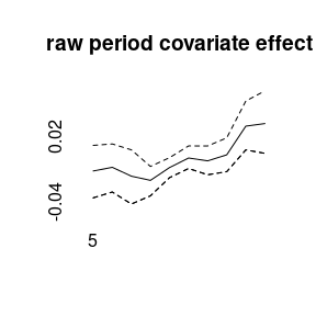
plot(model5)