Bayesian Age-Period-Cohort Prediction

Prediction

Because period and cohort effects are modelled as random walks, they can be extrapolated as a continuation of these trends, which lets predict_apc() forecast cases for years beyond the observed data. For a first introduction to bamp(), see vignette(“bamp”, package=“bamp”); for other model specifications, see vignette(“modeling”, package=“bamp”).

We use the bundled data example, which covers ten years:

data(apc)
plot(cases[,1],type="l",ylim=range(cases), ylab="cases", xlab="year", main="cases per age group")
for (i in 2:8)lines(cases[,i], col=i)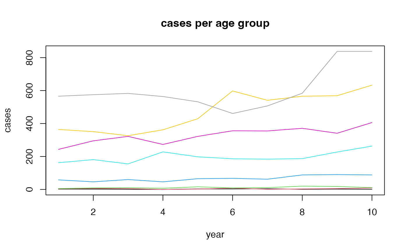

To see how well the forecast holds up against real data, we fit the model on only the first nine years and predict the tenth, so it can be compared to the cases actually observed that year.

model0 <- bamp(cases[-10,], population[-10,], age="rw1", period="rw1", cohort="rw1",
              periods_per_agegroup = 5)

predict_apc() extends the fitted model by the given number of periods. With update = TRUE the forecast is merged back into model0 (as model0$predicted) instead of being returned as a separate object:

model0<-predict_apc(object=model0, periods=1, population=population, update = TRUE)

The forecast for year 10 (dashed lines: 90% credible interval; solid line: median) lines up well with the true total cases (points), which were held out of the fit:

ts.plot(t(model0$predicted$cases_period), lty=c(2,1,2))
points(apply(cases,1,sum), pch=19)

The same credible intervals extend the period and cohort effects themselves into year 10:

ts.plot(t(model0$predicted$period), lty=c(2,1,2))

ts.plot(t(model0$predicted$cohort), lty=c(2,1,2))

Volker Schmid

2026-08-08

Prediction