
period=15:1
period[8:15]<-8:15
period<-period/5
period<-period-mean(period)
plot(period, type="l")

periods_per_agegroup=5
number_of_cohorts <- periods_per_agegroup*(10-1)+15
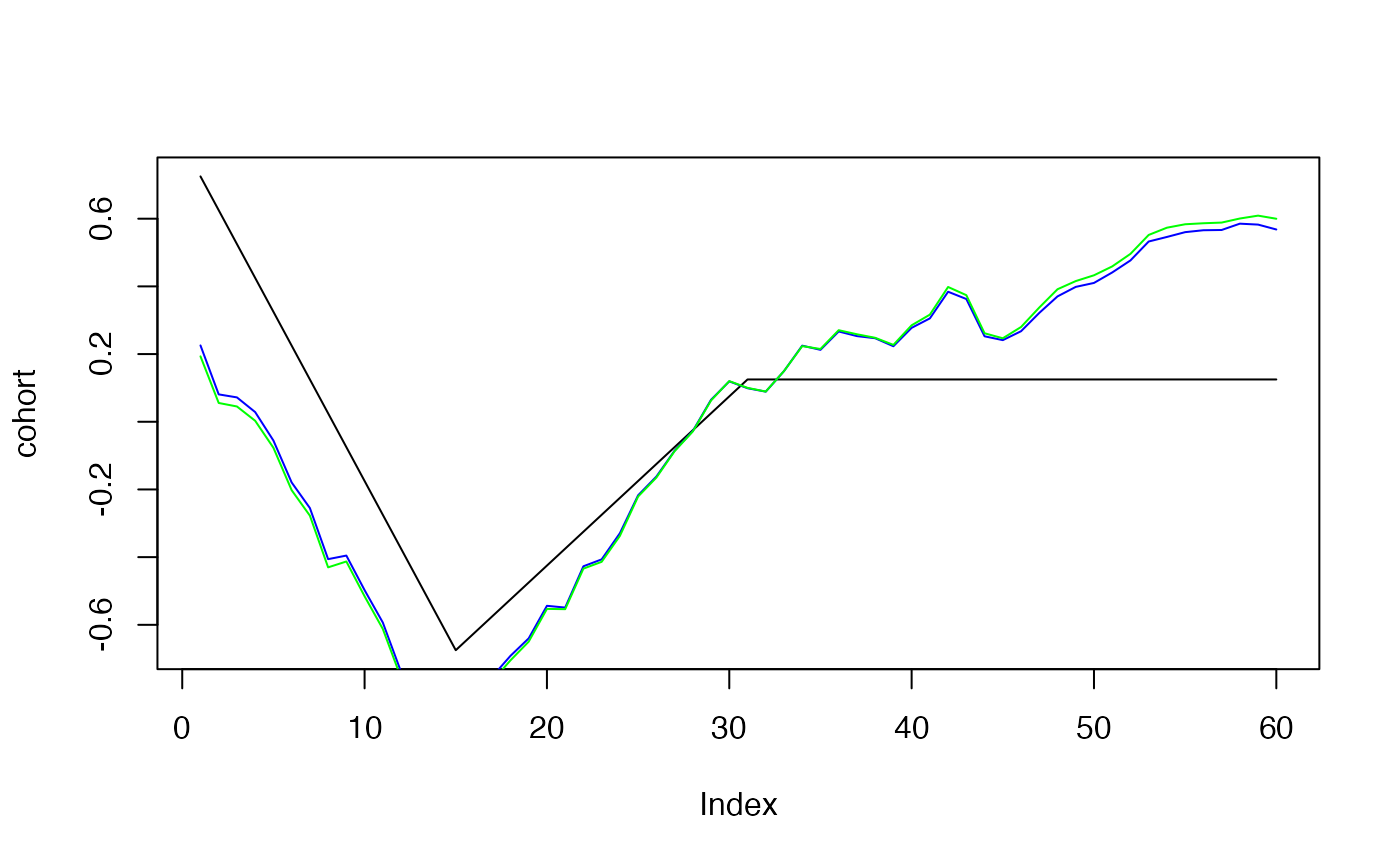
cohort<-rep(0,60)
cohort[1:15]<-(14:0)
cohort[16:30]<- (1:15)/2
cohort[31:60]<- 8
cohort<-cohort/10
cohort<-cohort-mean(cohort)
plot(cohort, type="l")

simdata<-apcSimulate(-10, age, period, cohort, periods_per_agegroup, 1e6)
print(simdata$cases)
##       [,1] [,2] [,3] [,4] [,5] [,6] [,7] [,8] [,9] [,10]
##  [1,]    0   10   22   52   85  114  172  413 1122  2991
##  [2,]    4    5   19   46   62   98  140  314  840  2246
##  [3,]    1    5   15   36   63   94  132  211  605  1646
##  [4,]    0    4    9   36   52   85  114  158  458  1232
##  [5,]    1    2    8   22   57   61   76  118  353   900
##  [6,]    1    0    7   22   25   56   90  122  264   653
##  [7,]    1    4    7   12   38   50   74   94  157   507
##  [8,]    0    0    8    7   40   51   61   81  147   393
##  [9,]    0    4   12   18   40   57   72  116  132   406
## [10,]    1    2    7   21   40   81  110  142  158   399
## [11,]    0    6   12   16   57   83  116  174  200   505
## [12,]    0    7    9   31   52   98  163  228  262   564
## [13,]    0   10   16   40   65  143  213  267  350   580
## [14,]    1   10   19   37   92  152  273  376  428   665
## [15,]    2    8   15   56  129  228  341  435  567   779
simmod <- bamp(cases = simdata$cases, population = simdata$population, age = "rw1",
period = "rw1", cohort = "rw1", periods_per_agegroup =periods_per_agegroup)
##
##  Model:
## age (rw1)  - period (rw1)  - cohort (rw1) model
## Deviance:     161.86
## pD:            48.89
## DIC:          210.75
##
##
##  Hyper parameters:                 5%           50%          95%
## age                              0.506        1.248        2.463
## period                          14.462       28.124       49.538
## cohort                          82.094      129.064      198.609
##
##
## Markov Chains convergence checked succesfully using Gelman's R (potential scale reduction factor).
## [1] TRUE


effects<-effects(simmod)
effects2<-effects(simmod, mean=TRUE)
#par(mfrow=c(3,1))
plot(age, type="l")
lines(effects$age, col="blue")
lines(effects2$age, col="green")

plot(period, type="l")
lines(effects$period, col="blue")
lines(effects2$period, col="green")

plot(cohort, type="l")
lines(effects$cohort, col="blue")
lines(effects2$cohort, col="green")
plot(prediction$cases_period[2,], ylim=range(prediction$cases_period),ylab="",pch=19)
points(prediction$cases_period[1,],pch="–",cex=2)
points(prediction$cases_period[3,],pch="–",cex=2)
for (i in 1:20)lines(rep(i,3),prediction$cases_period[,i])

plot(prediction$period[2,])

cov_p<-rnorm(15,period,.1)
simmod2 <- bamp(cases = simdata$cases, population = simdata$population, age = "rw1",
period = "rw1", cohort = "rw1", periods_per_agegroup = periods_per_agegroup,
period_covariate = cov_p)
##
##  Model:
## age (rw1)  - period (rw1)  - cohort (rw1) model
## Deviance:     161.96
## pD:            48.94
## DIC:          210.91
##
##
##  Hyper parameters:                 5%           50%          95%
## age                              0.526        1.224        2.436
## period                          14.251       28.022       48.707
## cohort                          82.016      130.447      201.982
##
##
## Markov Chains convergence checked succesfully using Gelman's R (potential scale reduction factor).
## [1] TRUE


